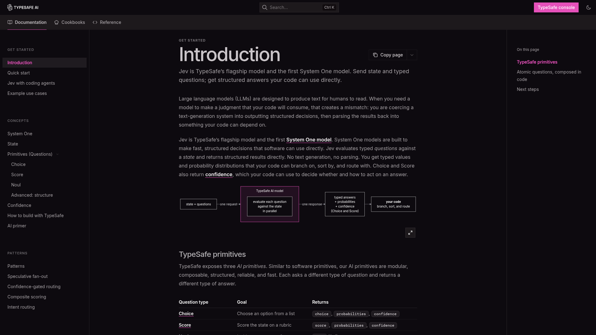
Jev AI Confidence Scores and RLCD: A Practical Guide

Jev AI’s launch materials emphasize calibrated probabilities alongside structured decisions. TypeSafe says its training method, Reinforcement Learning for Calibrated Decisions (RLCD), is designed to optimize for calibrated answers on “System One” tasks. That is a meaningful design goal, but a confidence value should never be treated as a guarantee that one particular prediction is correct.

Calibration is a property measured across a set of predictions. If a model assigns 0.8 confidence to many cases, roughly 80% of those cases should be correct for that confidence level to be well calibrated. A single score cannot verify that property by itself.

Confidence and correctness answer different questions

Correctness asks whether an individual decision matches the reference answer. Calibration asks whether groups of predictions with similar confidence are correct at the rate their confidence suggests. A system can be accurate but overconfident, or calibrated overall while still making an important error on one case.

For a support-routing model, a confidence of 0.9 is not a certificate that a billing issue belongs in the billing queue. It is a value whose meaning should be checked against labeled examples, especially for the current task, user population, and input distribution.

What TypeSafe says RLCD is for

TypeSafe contrasts RLCD with approaches such as reinforcement learning from human feedback and reinforcement learning from verifiable rewards. In the company’s framing, RLHF optimizes responses preferred by human raters, RLVR optimizes outputs that can be programmatically checked, and RLCD aims at calibrated decisions for software. These are concise descriptions from the launch announcement, not a full technical specification of the training method.

To understand exactly how Jev is trained, what calibration targets it uses, and which benchmarks apply, consult the original announcement and the latest documentation. Do not infer training details that TypeSafe has not published.

Jev System One Model, Clearly Explained: Fast Judgment and Eval · Sean’s AI Stories

A practical calibration test

Define a target: label what counts as correct for each possible output.
Separate development and test data: avoid tuning thresholds on the same examples used to report quality.
Bin predictions by confidence: compare average confidence with observed accuracy in each bin.
Track a proper scoring rule: use Brier score for probability predictions, alongside task-specific precision, recall, or ranking metrics.
Check slices: report results by language, channel, customer segment, and other relevant groups without exposing unnecessary personal data.
Recheck after change: refresh the evaluation when the model, schema, prompt-like question, or source data changes.

Expected calibration error can summarize the gap between confidence and observed accuracy across bins, but it depends on how the bins are selected and should not be the only metric. A reliability diagram makes overconfidence and underconfidence easier to inspect.

Use confidence to route, not to overrule safeguards

Once confidence is measured on a representative set, it can help route cases: accept routine, low-impact decisions; send uncertain cases to a review queue; and reject inputs outside the supported scope. Set thresholds by considering both error rates and the real cost of review. A threshold that saves time on product tagging may be inappropriate for payments, eligibility, or access control.

Record the threshold, the evaluation data, and who approved the policy. Do not silently treat “high confidence” as permission to bypass deterministic rules, privacy checks, or human approval requirements.

Structured output does not eliminate model error

Typed output can prevent some schema and parsing failures. It cannot guarantee that the semantic choice is correct, that the input contains enough information, or that a malicious string inside the input will be ignored. The surrounding application still needs input validation, constrained actions, audit logs, and a fallback.

Simon Willison’s review of Jev points readers to documented weaknesses involving numbers, dates, and adversarial content. This is exactly why a confidence value should be studied under edge cases, not only clean examples.

What others are saying about Jev AI

Willison’s assessment is both interested and cautious: he sees value in decision-shaped work such as classification and reranking, but raises the opacity of another black-box model and calls out known limitations. KDnuggets also notes that public information about Jev’s internal training and architecture is limited. Their shared implication is practical: measure confidence yourself and do not treat vendor terminology as a substitute for task-level evidence.

Frequently asked questions about Jev AI confidence

Does a Jev AI probability guarantee the decision is right?

No. A probability is a model output that must be evaluated for the intended task. Calibration is measured across groups of predictions, not guaranteed for every individual response.

What is RLCD?

TypeSafe expands RLCD as Reinforcement Learning for Calibrated Decisions and describes it as training for calibrated probabilities on structured decision tasks. The public launch post is the source for that description.

Which metrics should I use?

Use task-specific metrics such as precision, recall, and ranking quality, plus probability metrics such as Brier score and calibration plots when the output includes probabilities. Include slices and edge cases that reflect real use.

Sources and further reading

Start by defining what the confidence value refers to

A confidence score is not self-explanatory. Before using one in a workflow, write a sentence that says what the number is supposed to estimate. For a binary question, it might mean the probability that a labeled condition is true. For a choice, it might describe the probability assigned to the selected class. For an ordinal score, it may be a signal for ordering rather than a literal probability of anything. Those interpretations lead to different tests and different safety rules.

TypeSafe’s Jev announcement describes probabilities alongside structured decisions and introduces Reinforcement Learning for Calibrated Decisions, or RLCD. That public description establishes the intended direction, not the meaning of every score in every task. The current TypeSafe documentation should be the authority for the response contract and supported behavior. Your own evaluation must establish what the signal means on your data.

Calibration is a population property

Suppose a system assigns 0.7 probability to one class for 1,000 cases. A calibrated system would be correct on approximately 700 of those cases, allowing for ordinary statistical variation. That statement concerns the group, not any individual record. It does not mean that the next case with a 0.7 score has a 70 percent chance that a reviewer will agree, unless the target, sample, and evaluation design make that interpretation appropriate.

This distinction matters operationally. A case with a 0.95 score can still be wrong. A case with a 0.55 score can still be right. Calibration helps an organization set expectations and abstention policies across many decisions; it cannot turn an uncertain prediction into a guarantee. Treating confidence as certainty is especially dangerous when the model is exposed to a new language, a new product, or an input format absent from the evaluation set.

Accuracy and calibration answer different questions. Accuracy asks how often the selected answer matches the label. Calibration asks whether the stated probability tracks the observed frequency of correctness. Ranking quality asks whether higher-scored items tend to be better candidates than lower-scored items. A model may be strong on one property and weak on another, so do not compress all three into a single “quality” number.

Turn the decision into an evaluable target

Calibration cannot be measured until the team has a target label that independent reviewers can apply. Write the question in plain language, specify the observation window, and define what counts as a positive or negative outcome. “Will this ticket need escalation?” could mean escalation within 24 hours, escalation at any point in the case, or a reviewer’s immediate opinion. Choose one definition and use it consistently.

For multiclass decisions, list all permitted labels and write a short labeling guide. Include examples that distinguish neighboring categories, along with an explicit policy for ambiguous records. If two labels lead to the same downstream action, consider combining them. If the true answer can be outside the list, provide an abstention or review route rather than forcing a plausible-looking class.

For scores, document the meaning of each level and whether the scale is nominal, ordinal, or intended to approximate a probability. A relevance score of four out of five is not automatically an 80 percent chance of relevance. A score can be useful for prioritizing a queue while being unsuitable as a hard eligibility threshold. The contract should say which use is permitted.

Build a test set that represents decisions in time

Use examples that resemble the inputs the system will see after launch. Random samples are a reasonable starting point, but they can hide rare languages, unusual channels, long messages, and cases that humans already routed away from the normal process. Add a deliberate sample of ambiguous and difficult records. Keep the selection procedure and time range in the evaluation notes so a future team can reproduce it.

When labels depend on what happened later, respect the point at which the decision would have been made. Do not include a post-resolution note, a final status field, or a reviewer correction that would not have existed at inference time. Related messages from one case should remain in the same split; otherwise nearly identical records can make the test look more reliable than deployment will be.

Use a development set to refine the question and a separate validation set to choose thresholds or a calibration mapping. Preserve an untouched test set for the final estimate. If the examples are too few for stable conclusions, report that limitation instead of presenting a precise percentage. Confidence intervals, bootstrap estimates, or repeated time-based evaluations can communicate uncertainty more honestly than an extra decimal place.

Read a reliability diagram without being misled

A reliability diagram groups predictions into confidence bins. For each bin, plot average predicted confidence against the observed rate of correct decisions. The diagonal represents ideal calibration. Points below it indicate overconfidence: the model says 0.8, but the observed correctness is nearer 0.6. Points above it indicate underconfidence. Include the number of examples in every bin; a visually dramatic point based on three records should not carry the same weight as a point based on 3,000.

There is no single universally correct binning scheme. Equal-width bins make the horizontal axis easy to read, while equal-count bins can prevent sparse regions from dominating the chart. Compare more than one reasonable view for small data sets, and show uncertainty where possible. Calibration curves can become unstable at the extremes because there may be very few predictions near zero or one.

For multiple classes, decide whether you are evaluating the confidence of the chosen class, the full probability vector, or both. One-vs-rest diagrams can reveal a class that is overconfident even when the top-line diagram looks acceptable. Also examine the relationship between confidence and abstention: if the system is used only above a threshold, calibration among accepted cases may be more relevant than the average over all records.

Use Brier score carefully

For a binary target with outcome y equal to zero or one and predicted probability p, the Brier score is the average of (p - y)^2. Lower is better. It penalizes confident wrong predictions more heavily than cautious wrong predictions, which makes it useful when probability quality matters. Always compare it with a baseline, such as a predictor that assigns the historical positive rate to every case.

For several classes, calculate squared error over the probability assigned to each class and state the convention used. A multiclass Brier result is not directly interchangeable with a binary result. Compare the same label set, examples, and missing-data policy across Jev and every baseline. If a model returns scores rather than probabilities, do not call the metric a Brier score until the score has a defensible probabilistic interpretation.

Brier score combines discrimination and calibration. A lower value is encouraging, but it does not tell an operator which class fails, whether rare cases are safe, or what a false positive costs. Pair it with a confusion matrix, per-class results, reliability diagrams, and a decision-cost analysis. A small improvement in a global metric can be a poor trade if it causes severe errors in a low-volume but important group.

Understand ECE and its blind spots

Expected calibration error, often abbreviated ECE, usually averages the absolute difference between confidence and observed accuracy across bins. It is convenient for comparing runs, but it is not a measurement free of design choices. The number of bins, the bin boundaries, the treatment of empty bins, and the weighting rule all affect the result. Record those choices whenever ECE is reported.

ECE can hide local failures. A large common class may dominate the average while a rare class is badly overconfident. Overconfidence in one range and underconfidence in another can also look modest after aggregation. Use ECE as a summary, never as the only evidence. A table with bin counts and observed accuracy is often more actionable than a single score.

Post-hoc calibration can improve a model’s probabilities without changing its chosen labels. A temperature-like mapping, isotonic mapping, or another calibration method must be fitted on data separate from the final test set. The mapping can itself drift when the class mix or input population changes. Validate it again after significant changes to the decision question, traffic source, or model version.

Check calibration by class, subgroup, and time

Report support and error metrics for every class. In a support taxonomy, a rare billing label may have excellent overall accuracy while a neighboring account-access label receives systematically high confidence for the wrong records. Look at precision, recall, false-positive rate, false-negative rate, and confidence distributions together. For ordinal tasks, report how far errors move from the correct level; confusing adjacent ratings may have a different cost from a large jump.

Repeat the analysis across meaningful slices such as language, region, channel, account type, document format, or product generation. Use privacy-conscious aggregation and avoid publishing tiny cells that could identify people. A difference is a reason to investigate data coverage, label quality, or decision design; it is not by itself proof of the cause. Subgroup calibration may require enough observations to support a stable estimate.

Time is another subgroup. A model can be calibrated on last quarter’s tickets and overconfident after a policy change. Track confidence bands, correction rates, class mix, missing fields, and abstention over time. Use a rolling labeled sample to identify drift. When the label definition changes, treat it as a new task rather than comparing its metrics as though nothing changed.

Design selective prediction and abstention

Many useful deployments do not ask the model to decide every case. A selective policy accepts recommendations above a validated confidence threshold and sends the remainder to a person or a conservative fallback. Measure coverage, the proportion of records accepted automatically, and selective risk, the error rate among those accepted. Plot the trade-off instead of choosing a threshold because a round number feels safe.

A threshold should reflect the consequence of each error. A low-risk internal tag might justify broad coverage, while an account-access or payment action may require review regardless of confidence. Include the reviewer capacity and expected queue size in the policy. Otherwise a threshold that looks accurate in isolation can overload the human path and create delayed decisions.

Abstention must be observable. Record why an item was deferred: low confidence, missing field, unsupported category, timeout, or an application validation failure. These reasons point to different fixes. More examples may help the first case; input normalization may help the second; a revised taxonomy may help the third. Do not label every fallback a “model error.”

What RLCD can and cannot establish

TypeSafe presents RLCD as a reinforcement-learning approach intended to optimize calibrated decisions, in contrast with objectives centered on human preference or programmatically checkable answers. That is a claim about the company’s training goal and product framing. It does not establish that every Jev probability is calibrated on every task, language, subgroup, or distribution.

A training objective can be well designed while deployment behavior varies with the question definition and the evidence available in the input. Ask for reproducible task-specific evidence: what target was used, what data was held out, how calibration was measured, and how uncertainty was represented. If public material does not answer those questions, record the gap as an open evaluation item rather than filling it with assumptions.

Independent discussion can help put the claim in context. Simon Willison’s analysis treats decision models as a useful practical framing while calling attention to black-box limitations and difficult inputs. KDnuggets’ commentary is cautious about novelty and the amount of public technical detail. Neither is a benchmark of your workflow, but both reinforce the value of testing rather than inferring reliability from terminology.

Put safeguards around the score

Keep authorization, policy interpretation, and irreversible mutations outside the model. The application should verify that the returned decision belongs to the expected task and allowed values, then apply a separately reviewed action policy. A score should not grant access, send money, delete records, or contact a customer without the checks required by that domain.

Run a shadow period when possible. Let Jev produce recommendations while the existing process remains authoritative. Compare recommendations with the current path and with later adjudicated labels. Investigate disagreement slices instead of only counting agreement. When the evidence is adequate, enable one reversible action for a limited population, preserve a kill switch, and define the conditions that automatically return the workflow to review.

Log enough to investigate: task definition, model identifier, returned decision, confidence, threshold, action, latency, fallback reason, and later correction. Minimize raw personal data, set retention limits, and control access to evaluation records. A score without its decision context is difficult to audit and easy to misinterpret months later.

A repeatable confidence evaluation protocol

Write the target outcome, allowed decisions, abstention route, and error costs.
Assemble time-appropriate labeled examples, including ambiguous, rare, and out-of-scope cases.
Freeze a final test set before tuning thresholds or calibration mappings.
Run Jev and at least one simple, task-matched baseline on identical examples.
Report accuracy, per-class errors, reliability diagrams, Brier score, ECE definition, and subgroup results.
Measure coverage and selective risk for every proposed confidence threshold.
Test missing fields, distribution changes, adversarial text, timeouts, invalid responses, and fallback behavior.
Run in shadow mode, review disagreement, and define drift triggers before automatic action.

The protocol may conclude that Jev is a good fit, that another model is better, or that a deterministic rule should remain in place. Each conclusion is useful when it is tied to a clearly defined decision and evidence collected on the population that matters. Confidence scores become valuable not when they sound authoritative, but when the surrounding measurement and safeguards make their limits explicit.